Basics of Radiometric Correction for Hyperspectral Data
Summary
- Introduction
- Atmospheric Effects
- System Effects
- Radiometric Correction Models
- Python Code for a LOWTRAN7 Atmospheric Absorption Extinction Model
- References
Introduction
The atmosphere is all nice and necessary for daily life, but it sure does make it tricky to obtain picture perfect hyperspectral images taken by satellites. While we shake our fist at refraction, scattering, and absorption corrupting our data, we are simultaneously amazed at the blue sky produced by the same effects and make it a common theme in desktop wallpapers. We can't blame all our inadequacies on atmospheric effects though. Hyperspectral images also contain sensor errors such as striping, and smile and keystone artefacts which need correcting. These correction procedures require models as we shall see towards the end of this blog post.
There will be some referencecs to Hyperion data so let's understand that.
Hyperion Data
Hyperion is the first satellite hyperspectral imager on the Earth Observing-1 (EO-1 Satellite). This satellite was part of NASA's New Millennium Program Earth Observing series and sat in a sun-synchronous orbit1. The hyperspectral sensor had 220 spectral bands and a spatial resolution of 30 m. The images are taken via pushbroom which means stripes (with 7.5 km swath width in the case of Hyperion) are taken sequentially to build a 2D image with 220 channels.
Hyperion data is taken above the atmosphere so it will be affected by the atmosphere.
Atmospheric Effects
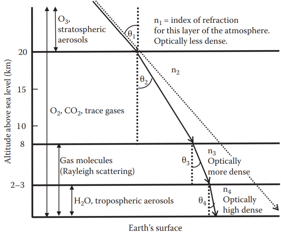
The atmosphere contains molecules such as water, carbon dioxide, ozone, and aerosols. These impede the path that light takes from the scene towards the imaging sensor. The major effects of the atmosphere are: refraction, scattering, and absorption.
Refraction
Refraction is the bending of light as it enters a medium with a different refractive index. It is refraction that makes a straw appear bent in a glass of water. Every medium has a refractive index $n$ defined as $$ n = c/v $$ where $c$ is the speed of light in vacuum and $v$ is the speed of light in the medium.
 {:width="80%"}
Scattering
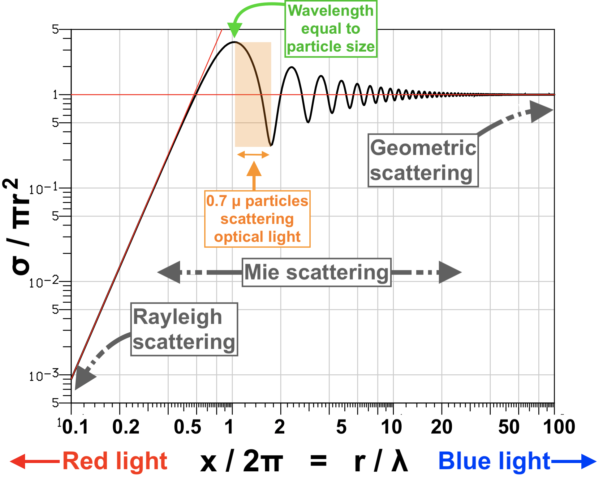
Atmospheric scatter is caused by many diffuse reflections of light off particles in the air. There are three regimes for scattering: Rayleigh, Mie, and optical depending on the ratio between the incident light wavelength and particle size. Rayleigh when the wavelength $\lambda$ is much smaller than the particle size $d$, optical when the wavelength is much larger than the particle size, and Mie inbetween Rayleigh and optical where there are resonances $0.1 < \lambda/d < 10$. This is aptly described in Figure 2.
 {:width="80%"}
Assuming Rayleigh scattering, the intensity $I$ of light scattered is given by $$ I = I_0\frac{1+\cos^2\theta}{2R^2}\left(\frac{2\pi}{\lambda}\right)^4 \left(\frac{n^2-1}{n^2+2}\right)^2 \left(\frac{d}{2}\right)^6 $$ where $I_0$ is the original intensity, $\theta$ is the scattering angle, and $R$ is the range to the distance to the particle (Seinfeld and Pandis 2006).
The scatter cross section $\sigma_s$, after averaging over all scatter angles (Cox et al. 2002), is given by $$ \sigma_s = \frac{2\pi^5 d^6}{3\lambda^4} \left(\frac{n^2-1}{n^2+2}\right)^2 .$$
You may also this relation with the polarisability $\alpha$ given by (Blue Sky 2015) $$ I = I_0 \frac{8\pi^4 \alpha^2}{\lambda^4 R^2}(1+\cos^2\theta) .$$
Shorter wavelengths are scattered more as can be seen by the $\lambda^{-4}$ dependence so when we look at the sky on a sunny day, we can see more of the shorter wavelength blue light compared to red light. However, if there is heavy air pollution (possibly from bushfires), blue light is scattered away leaving the red light.
Atmospheric Absorption
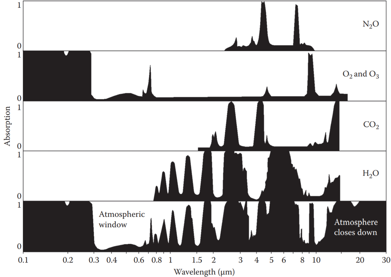
According to Gao et al. (2009), eight gases in the atmosphere have measureable absorption effects for hyperspectral imagers in the wavelength range 400--3000 nm with spectral resolution 1--20 nm. These gases are: water vapour H$_2$O, carbon dioxide CO$_2$, ozone O$_3$, nitrous oxide N$_2$O, carbon monoxide CO, methane CH$_4$, oxygen O$_2$, and nitrogen dioxide NO$_2$. Water is by far the most absorbing and this is illustrated in Figure 3.
 {:width="80%"}
Transmittance
Attenuation coefficient $\tau$ and extinction coefficient $\alpha$ $$ \tau_\lambda(z) = \int_0^z \alpha(\lambda,z) dz $$
$$ T(z,\theta) = e^{-\tau_\lambda(z)/\cos\theta} $$ where $\tau_\lambda$ consists of the contributions from Rayleigh scattering, and absorption from water and ozone. $\cos\theta$ accounts for oblique view.
System Effects
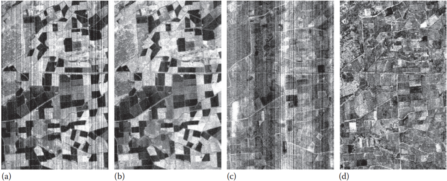
Striping Artefacts
Noticable columns that are brighter than adjacent columns
 {:width="80%"}
Sensor Artefacts
spectral and spatial errors on detector array due to optical aging, degradations, aberrations, and misalignments in pushbroom systems, especially in hyperspectral pushbroom systems where crosstrack and spectral pixels are continuously recorded at the same time using an area detector array.
Spectral error is smile, spatial error is keystone
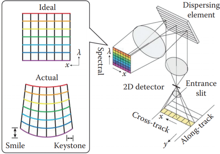 {:width="80%"}
Destriping for Land
Procedure by Goetz et al. (2003) great for terrestrial
pixel value (or digital number) $x_{ijk}$ for row $i$, column $j$, and band $k$ For each row $i$, we multiply by gain $a_{jk}$ and offset $b_{jk}$ such that each row's mean $\mu_{jk}$ and standard deviation $\sigma_{jk}$ is equal to the overall channel's mean $\mu_k$ and standard deviation $\sigma_k$. $$ x_{ijk}' = a_{jk}x_{ijk} + b_{jk} $$
$$ a_{jk} = \frac{\sigma_k}{\sigma_{jk}} $$
$$ b_{jk} = \mu_k - \frac{\sigma_k}{\sigma_{jk}} \mu_{jk} $$
This is applied Hyperion in Figure 4.
Maximum Noise Fraction
like PCA based on noise covariance
Destriping for Water
Water absorbs too much compared to land. Need to try something different. Enter
Vertical Radiance Correction (VRadCor)
uses both spatial and spectral info $$ R_i' (\lambda_k) = a_i(\lambda_k) R_i(\lambda_k) + b_i(\lambda_k)$$
Correcting Smile and Keystone Errors
For smile, calibrate with absorption lines assume spectral shift is linear across array
Integration, cubic spline method
Radiometric Correction Models
$L_{obs}$ at sensor radiance, $L_a$ path radiance, $T_2$ sun-surface-sensor two way transmittance, $S$ spherical albedo, $E_s$ exoatmospheric solar irradiance, $\theta_s$ solar zenith angle, $\rho$ surface reflectance.
$$ L_{obs} = L_a + \frac{T_2 \rho}{1-\rho S}\frac{E_s\cos\theta_s}{\pi} $$
$$ \rho = \frac{L_{obs}-L_a}{(L_{obs}-L_a)S+T_2 E_s\cos\theta_s/\pi} $$
Absolute Correction
MODTRAN
Moderate Resolution Atmospheric Radiance and Transmittance Model
6S
Second Simulation of the Satellite Signal in the Solar Spectrum
FLAASH
Fast Line-of-sight Atmospheric Analysis of Spectral Hypercubes
ELC
Empirical Line Calibration
linear regression against lab spectra, need to know materials in FOV.
ATREM
Atmospheric Removal
ATCOR
Atmospheric Correction
HATCH
High-accuracy Atmospheric Correction for Hyperspectral data
Comparison
No idea
Relative Correction
same scene taken on different dates, normalised to reduce variations
!pip install lowtran
# from https://github.com/space-physics/lowtran/blob/master/ScatterRadiance.py
scatterRadiance()
References
1. Pu, R. (2017). Hyperspectral remote sensing: Fundamentals and practices. CRC Press.↩
2. Modified from Miller, S. W., and Vermote, E., NPOESS Visible/Infrared Imager/Radiometer: Algorithm Theoretical Basis Document, Version 5, Raytheon, Lanham, Maryland, 2002.↩
4. From Jensen, J. R., Remote Sensing of the Environment: An Earth Resource Perspective, 2nd ed., Pearson Education, Inc., New York, 2007.↩
5. ©2003 IEEE. From Goetz, A. F. H., Kindel, B. C., Ferri, M., and Qu, Z., IEEE Transactions on Geoscience and Remote Sensing, 41, 1215−1221, 2003↩
6. Yokoya, N. et al., Applied Optics, 49(24), 4568–4575, 2010.↩
7. ↩